Matlab files:
(Right click or left click and use the `File' menu to download. Octave is a free equivalent to Matlab.)
| MethodI.m |
| MethodII.m |
| EstimateVariance.m |
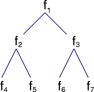
plus a simulated data set (datatree.dat) of a 7 generation lineage tree with 3 measurements per cell. Each row of the data is from one cell, with row number corresponding to the subscripts in the figure below (only a 3 generation tree is shown).
Example
To load the example data, type in Matlab:
>> f= load('datatree.dat');
To run Method I, type:
>> MethodI(f)
The estimate for the fluorescence conversion factor should be 29.9.
For Method II, the suspected range of the fluorescence conversion factor and of the measurement error must be specified:
>> nu= 10:2:60;
>> sig= 40:5:60;
The posterior probability is calculated on a mesh specified by these values:
>> s= MethodII(f, nu, sig);
The default is to return -log(posterior probability). To sketch the result:
>> contour(sig, nu, exp(s-max(max(s))), 10)
>> xlabel('measurement error'); ylabel('\nu');
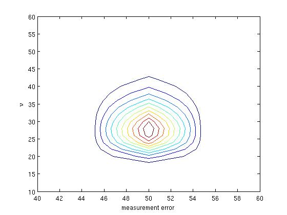
where we have used a normalization factor, exp(-max(max(s))), to prevent numerical underflow. For this simulated data, the true value of the measurement error is 50 and the conversion factor is 25.
An estimate of the measurement error, which helps sets the range required by Method II, is given by:
>> sqrt(EstimateVariance(f))
The estimate should be 49.3.